A regression line (or line of best fit) can be added to any scatter plot with numerical X and Y axes, to allow you to:
- Visualize how well your data fits an equation for a correlation between two variables
- See a statistical calculation of how well the equation fits
Here is an example of a dataset plotting number of cases of a disease against time. Check the box (which appears whenever you have a graph with a numeric X and Y) to add the regression line:
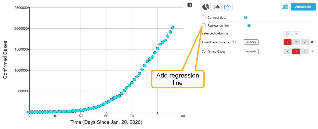
If the box is not visible, then you may not have a numeric/numeric plot, it may have been hidden, or you may have selected Connect dots instead.
By default, the line drawn will be a Linear equation:
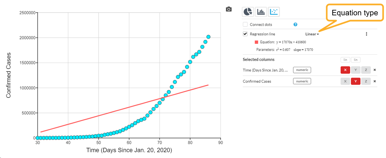
You can select other equation types from the selector. Available options are Linear, Quadratic, Cubic (3rd order), Exponential, Logarithmic, Power and Logistic. Here is the same graph with an Exponential regression.
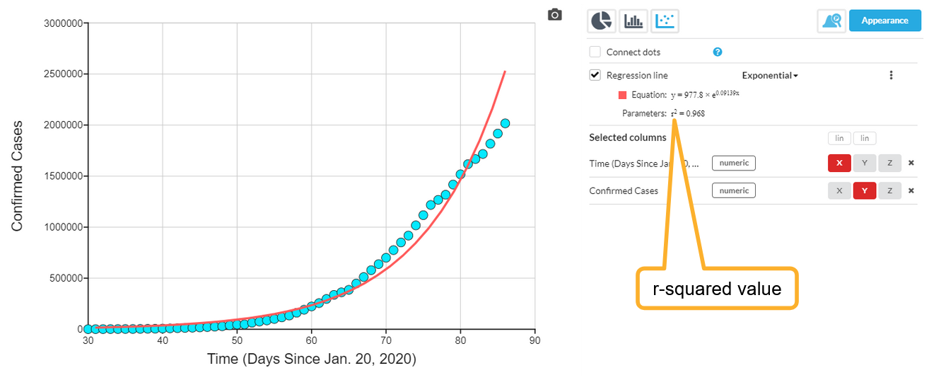
The actual equation is shown, along with the r2 (r-squared) value which tells you how well the equation fits your data (where 1.000 would be a perfect fit).
You can customize the look of the line, see the article on Customizing the appearance of the graph
Spearman's Rho (Spearman's Rank)
For linear regression, the value of Spearman's rank correlation coefficient ρ (rho) is also displayed. This correlation coefficient indicates the degree of correlation for variables that are not necessarily linearly related, but are have a monotonic relationship. Read more here on Wikipedia.
Regression line intercepts
You can see the X intercept and Y intercept values for a linear regression line together with the equation. However, if the intercept point of interest is not within the range of the auto-scaled axes, you can fix the axis extents and the regression line will extend as far as you have specified. Here is an example with the X axis extended to include the X intercept:
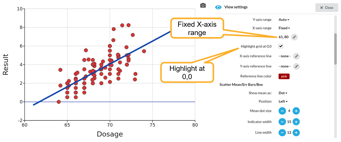
The Highlight grid at 0,0 option has also been used to provide a visual reference.
Additional regression options
Additional options for the regression line are found through the "3 dots" menu:
 These include Residuals and slopes and Forcing a linear regression line through the origin.
Forcing a linear regression through the origin (0,0)
Sometimes you know that there are some physical laws that mean that a linear relationship you are looking at will pass through the point at 0,0. For example, if you are looking at current vs voltage, you know that with no voltage, the current will also be exactly zero. You can add this knowledge to the linear regression calculation by selecting this checkbox:

This will then result in a linear equation of the form y = mx, rather than y = mx + c.
Extend regression line to fill X axis
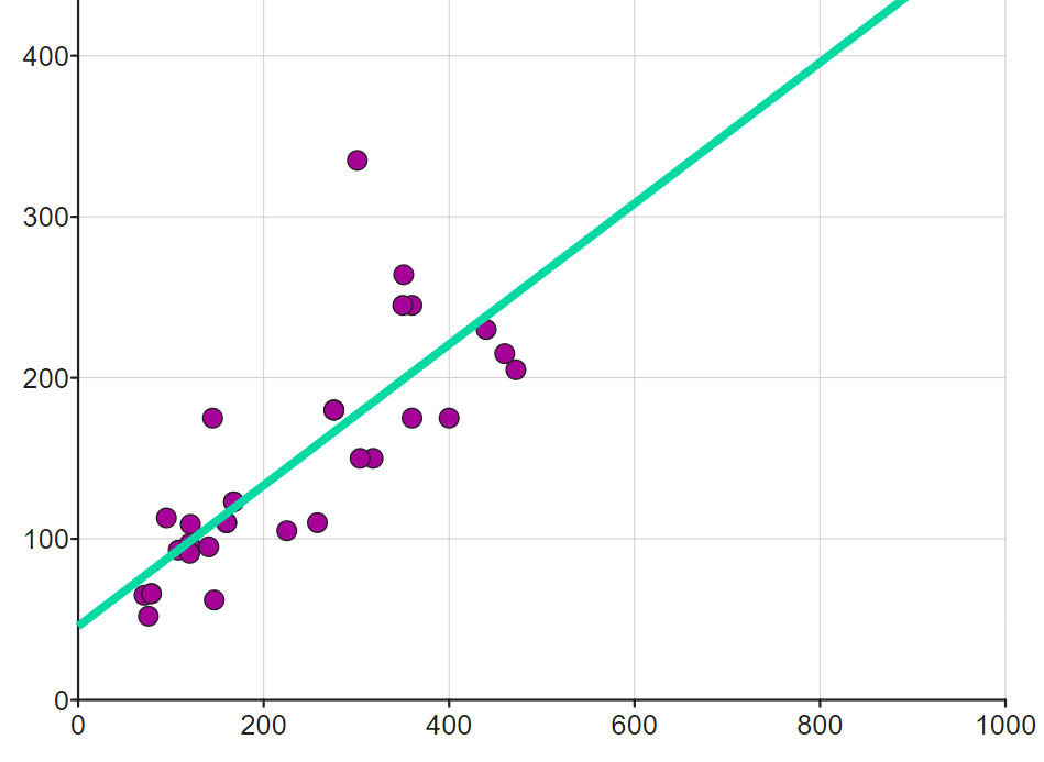
If you want the regression line to extrapolate beyond your data and fill the entire axis - for example if you have customized your axis extent - then you can check the Extend line to fill extended X axis option.

The regression line will then fill the entire X axis, and the Y axis will also be extended if required to show the complete line.
See also
Working with residuals and slopes